How models learn the price of thinking more

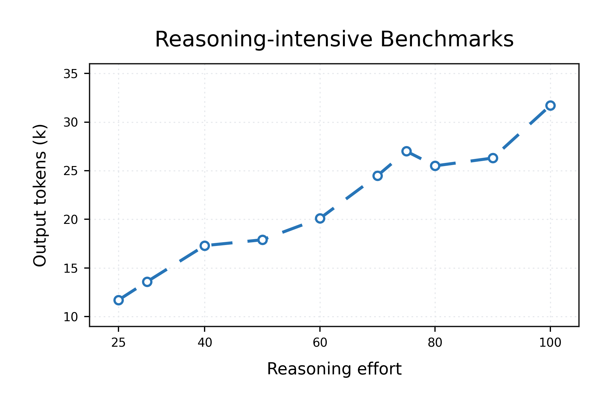
Something very interesting about some of DeepSeek V4.1’s benchmarks is that output length seems to grow very close to linearly with reasoning effort. If you’ve read my previous article, you’re probably familiar with the idea that reasoning efforts are often passed as scalar values to models, and this is the case for DeepSeek as well: it has an effort setting from 1 to 100. But there’s no fundamental reason that moving from 50 to 60 should add about the same amount of computation as going from 80 to 90.

DeepSeek-V4.1-Flash output length across reasoning-effort values on reasoning-intensive benchmarks — Figure 1. In DeepSeek-V4.1-Flash, average output length increases with reasoning effort, close to linearly in reasoning-intensive benchmarks. Source: DeepSeek-V4.1-Flash Technical Report.

It turns out that this property is closely related to how DeepSeek defines its RL reward. There’s also a cool connection to Cognition’s SWE-2, which was also released today. Essentially, reasoning effort is a way of choosing the price of test-time compute, and we can think of DeepSeek V4.1’s RL penalty as mapping user-facing effort to compute prices, and Cognition SWE-2’s as thinking about what compute price should be at a particular point (based on performance / Pareto frontier).

Simple model

Consider a very simple model, where for a specific problem, a model spends \(\ell\) reasoning tokens, and \(p(\ell)\) is the probability of solving the problem given we spent this many tokens. Then suppose each additional reasoning token has cost \(\mu\) in our reward. We can think of our model as optimizing

U(\ell) = p(\ell) - \mu \ell

(although obviously RL doesn’t directly optimize the reward which isn’t directly differentiable in the model weights, but this is a good abstraction). If we differentiate this with respect to \(\ell\) we get

U'(\ell) = p'(\ell) - \mu.

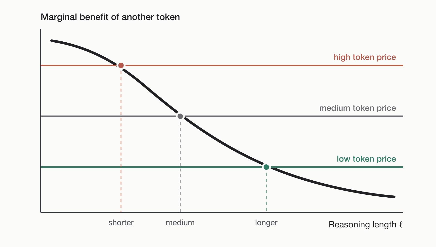
So at an optimum in the interior \(\ell^\star\), we have \(U^{\prime}(\ell^\star) = 0 \implies p^{\prime}(\ell^\star) = \mu\). The takeaway is: the model should keep thinking, until the expected marginal benefit of another reasoning token falls to exactly the “price” of that token. This is the standard Lagrangian picture that you would learn in a convex optimization class, i.e. if we wanted to maximize expected performance under a compute budget

\max_{\ell \ge 0}\ p(\ell) \quad \text{subject to} \quad \ell \le B

then the Lagrangian would contain the term \(-\mu \ell\) where the multiplier \(\mu\) is the shadow price of compute (how much one additional unit of compute is worth, at the optimum).

DeepSeek V4.1: effort is log scale for token price

During RL, DeepSeek V4.1 conditions the policy on effort values \(b\) from \(1\) to \(100\). It adds a length penalty

r_{\mathrm{len}}(\ell,b) = -\min\left\{ C_{\max}, k(b)\frac{\ell}{L_{\mathrm{norm}}} \right\},

with

k(b) = k_0 \exp\left( -\frac{b-b_{\min}}{\tau} \right),

meaning that the penalty coefficient decreases exponentially with effort. So the effective price of a reasoning token (ignoring the cap), is then \(\mu(b) \propto \exp\left(-\frac{b}{\tau}\right).\) So every additive increase in the effort number makes reasoning multiplicatively cheaper. We can also rewrite this as \(b=\text{constant}-\tau\log\mu\), so we can think of the reasoning number \(b\) as approximately a log coordinate for the price of reasoning compute.

DeepSeek then makes the assumption (in Appendix C of the report) that the marginal benefit of more reasoning falls roughly exponentially, i.e. \(p^{\prime}(\ell) \approx a e^{-\ell/s}.\) At the optimum reasoning length \(\ell^\star\), we have

p'(\ell^\star) = \mu(b)

a e^{-\ell^\star/s} = \frac{k_0}{L_{\mathrm{norm}}} e^{-(b-b_{\min})/\tau}

and taking logs we get

\ell^\star(b) = s\log\left(\frac{aL_{\mathrm{norm}}}{k_0}\right) + \frac{s}{\tau}(b-b_{\min}) \approx A+Bb.

The tldr is: if we assume exponentially diminishing returns to thinking, and exponentially decreasing token price, then this gives \(\approx\) linear reasoning length as a function of effort. (Just to be clear, this is about reasoning/output length rather than performance.)

A smaller effective per-token RL penalty intersects a decreasing marginal-benefit curve at a longer reasoning length — Figure 2. Try changing the reasoning effort! The intersection’s x-coordinate is the optimal reasoning length. See how the reasoning effort toggle and this x-coordinate vary \(\approx\) linearly when you move it around.

Cognition SWE-2: what should the price of compute be?

Cognition uses a pretty similar objective in SWE-2:

R = S - \lambda_e C

where \(S\) = success, \(C\) = rollout cost, and \(\lambda_e\) is a cost penalty depending on effort \(e\). The interesting question here is how to choose \(\lambda_e\).

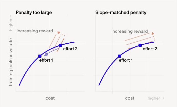
Suppose the base model has a Pareto frontier (cost-performance) \(s = f(c)\). Then for a fixed expected reward \(J = s - \lambda c\), the slope of the iso-reward lines (\(s = \lambda c + J\)) is \(\lambda\).

If \(m = f^{\prime}(c)\) is the local slope of the existing Pareto frontier, then a small movement along that frontier gives \(\Delta s \approx m \Delta c\) so \(\Delta J \approx (m - \lambda) \Delta c\). Cognition chooses \(\lambda = m\) so that moving slightly along the old frontier gives \(\approx 0\) reward improvement.

Why? If the cost penalty were larger, RL could try to “improve” an old high-effort policy by just making it cheaper and less capable, so that it behaves like a lower-effort policy (i.e. move down along the existing frontier), or vice versa. By having the reward line be tangent to the old frontier, this method encourages RL to improve/push the frontier outward instead.

Cognition SWE-2 diagram comparing an excessive cost penalty with a slope-matched penalty — Figure 3. With too large a penalty, reward can improve by sliding down the old frontier, so they match penalty to the frontier's local slope. Source: Cognition, “Introducing SWE-2”.

Overall takeaway

Okay so what’s the overall takeaway here? What does any of this actually mean?

So recall where I said that the marginal value of more compute should be equal to the shadow price of compute. DeepSeek basically asks, how should this effort number (which users can control) map to that price? And their answer is \(\text{price}(b)\propto e^{-b/\tau}\) which means that under exponentially diminishing returns, reasoning length should be \(\approx\) linear in effort. And this is what we see in their benchmark graphs!

Cognition instead cares about this question: what should this price be at a specific operating point? And their answer is,

\text{price} = \text{local slope of the base model's Pareto frontier}

which encourages RL to improve and push out the Pareto frontier rather than getting easy reward by sliding down the existing frontier.

Also their ideas of “cost” are a bit different too: DeepSeek just focuses on reasoning token length, while Cognition uses a combination of inference cost and rollout time.

The even more general takeaway is that “reasoning effort” is a pretty complicated thing, and even though you just see “low medium high”, there’s a real optimization problem behind all this. The objective is to teach the model a policy corresponding to asking “what is the value/cost of additional thinking?” so that the model can spend more compute (i.e. another token, step, detour, or subagent, etc!) when useful and worth it, without teaching it to waste tokens or collapse unnecessarily to a cheaper policy.

Simple model

DeepSeek V4.1: effort is log scale for token price

Cognition SWE-2: what should the price of compute be?

Overall takeaway

Sources